12 Z-scores
Z-scores are a handy way to standardize numbers so you can compare things across groupings or time. In this class, we may want to compare teams by year, or era. We can use z-scores to answer questions like who was the greatest X of all time, because a z-score can put them in context to their era.
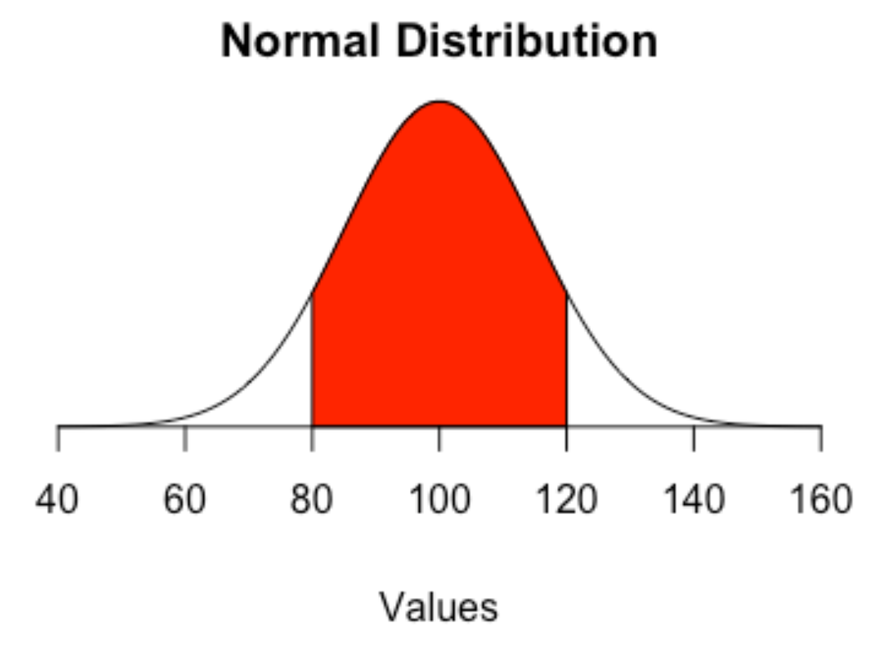
A z-score is a measure of how a particular stat is from the mean. It’s measured in standard deviations from that mean. A standard deviation is a measure of how much variation – how spread out – numbers are in a data set. What it means here, with regards to z-scores, is that zero is perfectly average. If it’s 1, it’s one standard deviation above the mean, and 34 percent of all cases are between 0 and 1.
If you think of the normal distribution, it means that 84.3 percent of all case are below that 1. If it were -1, it would mean the number is one standard deviation below the mean, and 84.3 percent of cases would be above that -1. So if you have numbers with z-scores of 3 or even 4, that means that number is waaaaaay above the mean.
So let’s use last year’s men’s college basketball season to see how we can use z-scores to rank teams. We’ll use a few stats that we think represent team quality: shooting percentage and rebounding margin, both for the team and their opponents. We’ll then combine those z-scores into a composite score.
12.1 Calculating a Z score in R
For this we’ll need the logs of all college basketball games last season.
For this walkthrough:
Load the tidyverse.
library(tidyverse)And load the data.
gamelogs <- read_csv("data/logs25.csv")Rows: 11962 Columns: 60
── Column specification ────────────────────────────────────────────────────────
Delimiter: ","
chr (10): Season, GameType, TeamFullName, Opponent, HomeAway, W_L, OT, URL,...
dbl (49): Game, TeamScore, OpponentScore, TeamFG, TeamFGA, TeamFGPCT, Team3...
date (1): Date
ℹ Use `spec()` to retrieve the full column specification for this data.
ℹ Specify the column types or set `show_col_types = FALSE` to quiet this message.The first thing we need to do is select some fields we think represent team quality and a few things to help us keep things straight. So I’m going to pick shooting percentage, rebounding and the opponent version of the same two:
teamquality <- gamelogs |>
  select(Conference, Team, TeamFGPCT, TeamTotalRebounds, OpponentFGPCT, OpponentTotalRebounds)
And since we have individual game data, we need to collapse this into one record for each team. We do that with … group by and summarize.
teamtotals <- teamquality |>
  group_by(Conference, Team) |>
  summarise(
    FGAvg = mean(TeamFGPCT),
    ReboundAvg = mean(TeamTotalRebounds),
    OppFGAvg = mean(OpponentFGPCT),
    OffRebAvg = mean(OpponentTotalRebounds)
    )
`summarise()` has grouped output by 'Conference'. You can override using the
`.groups` argument.To calculate a z-score in R, the easiest way is to use the scale function in base R. To use it, you use scale(FieldName, center=TRUE, scale=TRUE). The center and scale indicate if you want to subtract from the mean and if you want to divide by the standard deviation, respectively. We do.
When we have multiple z-scores, it’s pretty standard practice to add them together into a composite score. That’s what we’re doing at the end here with TotalZscore. Note: We have to invert OppZscore and OppRebZScore by multiplying it by a negative 1 because the lower someone’s opponent number is, the better.
teamzscore <- teamtotals |>
  mutate(
    FGzscore = as.numeric(scale(FGAvg, center = TRUE, scale = TRUE)),
    RebZscore = as.numeric(scale(ReboundAvg, center = TRUE, scale = TRUE)),
    OppZscore = as.numeric(scale(OppFGAvg, center = TRUE, scale = TRUE)) * -1,
    OppRebZScore = as.numeric(scale(OffRebAvg, center = TRUE, scale = TRUE)) * -1,
    TotalZscore = FGzscore + RebZscore + OppZscore + OppRebZScore
  )
So now we have a dataframe called teamzscore that has 360 basketball teams with Z scores. What does it look like?
head(teamzscore)# A tibble: 6 × 11
# Groups: Conference [1]
Conference Team FGAvg ReboundAvg OppFGAvg OffRebAvg FGzscore RebZscore
<chr> <chr> <dbl> <dbl> <dbl> <dbl> <dbl> <dbl>
1 A-10 MBB Davidson 0.455 30.2 0.449 31.3 0.561 -1.18
2 A-10 MBB Dayton 0.461 30.9 0.441 30.0 0.808 -0.780
3 A-10 MBB Duquesne 0.433 31.5 0.436 29.7 -0.532 -0.474
4 A-10 MBB Fordham 0.424 33.6 0.472 32.6 -0.946 0.638
5 A-10 MBB George Mason 0.459 33.0 0.386 29.6 0.721 0.292
6 A-10 MBB George Wash… 0.446 31.3 0.424 32.1 0.0873 -0.596
# ℹ 3 more variables: OppZscore <dbl>, OppRebZScore <dbl>, TotalZscore <dbl>A way to read this – a team with a TotalZScore of 0 is precisely average. The larger the positive number, the more exceptional they are. The larger the negative number, the more truly terrible they are.
So who are the best teams in the country?
teamzscore |> arrange(desc(TotalZscore))# A tibble: 361 × 11
# Groups: Conference [31]
Conference Team FGAvg ReboundAvg OppFGAvg OffRebAvg FGzscore RebZscore
<chr> <chr> <dbl> <dbl> <dbl> <dbl> <dbl> <dbl>
1 ACC MBB Duke 0.495 35.5 0.385 27.4 2.25 1.65
2 Ivy MBB Yale 0.490 35.0 0.410 28.7 1.18 1.24
3 OVC MBB Tenness… 0.463 37.5 0.419 30.9 1.81 2.10
4 WAC MBB Utah Va… 0.467 35.2 0.415 29.7 1.68 1.33
5 Big West MBB Cal Sta… 0.469 35.9 0.405 27.9 1.14 1.82
6 Summit MBB South D… 0.473 37.0 0.425 28 0.786 1.60
7 WCC MBB Saint M… 0.452 36.4 0.413 26.1 -0.140 1.97
8 Big South MBB High Po… 0.495 33.2 0.427 27.9 1.69 0.717
9 WCC MBB Gonzaga 0.500 34.6 0.413 28.9 1.57 1.14
10 CAA MBB UNC Wil… 0.469 36.1 0.431 27.9 1.30 1.63
# ℹ 351 more rows
# ℹ 3 more variables: OppZscore <dbl>, OppRebZScore <dbl>, TotalZscore <dbl>Don’t sleep on Tennessee State! If we look for Power Five schools, Duke and UConn are at the top, which checks out.
But closer to home, how is Maryland doing?
teamzscore |>
  filter(Conference == "Big Ten MBB") |>
  arrange(desc(TotalZscore)) |>
  select(Team, TotalZscore)
Adding missing grouping variables: `Conference`# A tibble: 18 × 3
# Groups: Conference [1]
Conference Team TotalZscore
<chr> <chr> <dbl>
1 Big Ten MBB Michigan State 4.36
2 Big Ten MBB Michigan 3.37
3 Big Ten MBB Illinois 2.97
4 Big Ten MBB Maryland 1.72
5 Big Ten MBB Purdue 1.60
6 Big Ten MBB UCLA 1.16
7 Big Ten MBB Southern California 0.661
8 Big Ten MBB Wisconsin 0.385
9 Big Ten MBB Indiana 0.338
10 Big Ten MBB Oregon -0.0226
11 Big Ten MBB Ohio State -0.0662
12 Big Ten MBB Penn State -0.0993
13 Big Ten MBB Nebraska -0.785
14 Big Ten MBB Northwestern -2.06
15 Big Ten MBB Minnesota -2.51
16 Big Ten MBB Iowa -3.40
17 Big Ten MBB Rutgers -3.48
18 Big Ten MBB Washington -4.13 So, as we can see, with our composite Z Score, Maryland is above average; good but not great. But better than most of their conference rivals. Notice how, by this measure, Michigan State and Michigan are far ahead of most of the conference, with Illinois in third.
We can limit our results to just Power Five conferences plus the Big East:
powerfive_plus_one <- c("SEC MBB", "Big Ten MBB", "Pac-12 MBB", "Big 12 MBB", "ACC MBB", "Big East MBB")
teamzscore |>
  filter(Conference %in% powerfive_plus_one) |>
  arrange(desc(TotalZscore)) |>
  select(Team, TotalZscore)
Adding missing grouping variables: `Conference`# A tibble: 79 × 3
# Groups: Conference [5]
Conference Team TotalZscore
<chr> <chr> <dbl>
1 ACC MBB Duke 8.21
2 ACC MBB Southern Methodist 4.83
3 Big East MBB Connecticut 4.66
4 Big 12 MBB Arizona 4.52
5 Big 12 MBB Houston 4.43
6 Big Ten MBB Michigan State 4.36
7 SEC MBB Florida 4.25
8 SEC MBB Tennessee 3.43
9 Big East MBB St. John's (NY) 3.38
10 Big Ten MBB Michigan 3.37
# ℹ 69 more rowsThis makes a certain amount of sense: three of the Final Four teams - Duke, Houston and Florida - are in the top 10. Auburn, the fourth team, ranks 16th. SMU is an interesting #2 here. It doesn’t necessarily mean they were the second-best team, but given their competition they shot the ball and rebounded the ball very well.
12.2 Writing about z-scores
The great thing about z-scores is that they make it very easy for you, the sports analyst, to create your own measures of who is better than who. The downside: Only a small handful of sports fans know what the hell a z-score is.
As such, you should try as hard as you can to avoid writing about them.
If the word z-score appears in your story or in a chart, you need to explain what it is. “The ranking uses a statistical measure of the distance from the mean called a z-score” is a good way to go about it. You don’t need a full stats textbook definition, just a quick explanation. And keep it simple.
Never use z-score in a headline. Write around it. Away from it. Z-score in a headline is attention repellent. You won’t get anyone to look at it. So “Tottenham tops in z-score” bad, “Tottenham tops in the Premiere League” good.