14 Simulations

On Feb. 21, 2023, fans of Maryland women’s basketball got a show from Brinae Alexander. The graduate transfer guard hit 6 of 9 three-pointers in a 96-68 destruction of Iowa (Caitlin Clark scored 18, her second-lowest output of the season). It was glorious.

But how rare was it? Did Alexander get lucky that night?

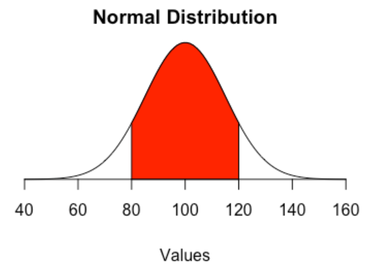
Luck is something that comes up a lot in sports. Is a team lucky? Or a player? One way we can get to this, we can get to that is by simulating things based on their typical percentages. Simulations work by choosing random values within a range based on a distribution. The most common distribution is the normal or binomial distribution. The normal distribution is where the most cases appear around the mean, 66 percent of cases are within one standard deviation from the mean, and the further away from the mean you get, the more rare things become.

Let’s simulate 10 three point attempts (0-9 makes) 1000 times with Alexander’s season long shooting percentage and see if this could just be random chance or something else.

We do this using a base R function called rbinom or binomial distribution. So what that means is there’s a normally distributed chance that Brinae Alexander is going to shoot above and below her season three point shooting percentage. If we randomly assign values in that distribution 1000 times, how many times will it come up 6, like this example?

First, we’ll load the tidyverse

library(tidyverse)

── Attaching core tidyverse packages ──────────────────────── tidyverse 2.0.0 ──
✔ dplyr     1.1.0     ✔ readr     2.1.4
✔ forcats   1.0.0     ✔ stringr   1.5.1
✔ ggplot2   3.4.1     ✔ tibble    3.1.8
✔ lubridate 1.9.2     ✔ tidyr     1.3.0
✔ purrr     1.0.1     
── Conflicts ────────────────────────────────────────── tidyverse_conflicts() ──
✖ dplyr::filter() masks stats::filter()
✖ dplyr::lag()    masks stats::lag()
ℹ Use the conflicted package (<http://conflicted.r-lib.org/>) to force all conflicts to become errors

set.seed(1234)

simulations <- rbinom(n = 1000, size = 10, prob = .439)

table(simulations)

simulations
  0   1   2   3   4   5   6   7   8   9 
  5  21  82 177 235 234 130  82  30   4

How do we read this? The first row and the second row form a pair. The top row is the number of shots made. The number immediately under it is the number of simulations where that occurred.

So what we see is given her season-long shooting percentage, it’s not out of the realm of randomness that she’d make 6 of those 9 attempts. In 1000 simulations, it comes up 130 times. So more than one time in 10, Brinae Alexander will go 6-9 from deep. More likely, she’d hit 4 or 5 of those attempts.

14.1 Cold streaks

During the final regular-season game in the 2021-22 season, Maryland’s men’s team, shooting .326 on the season from behind the arc, went 1-15 in the first half. How strange is that?

set.seed(1234)

simulations <- rbinom(n = 1000, size = 15, prob = .326)

hist(simulations)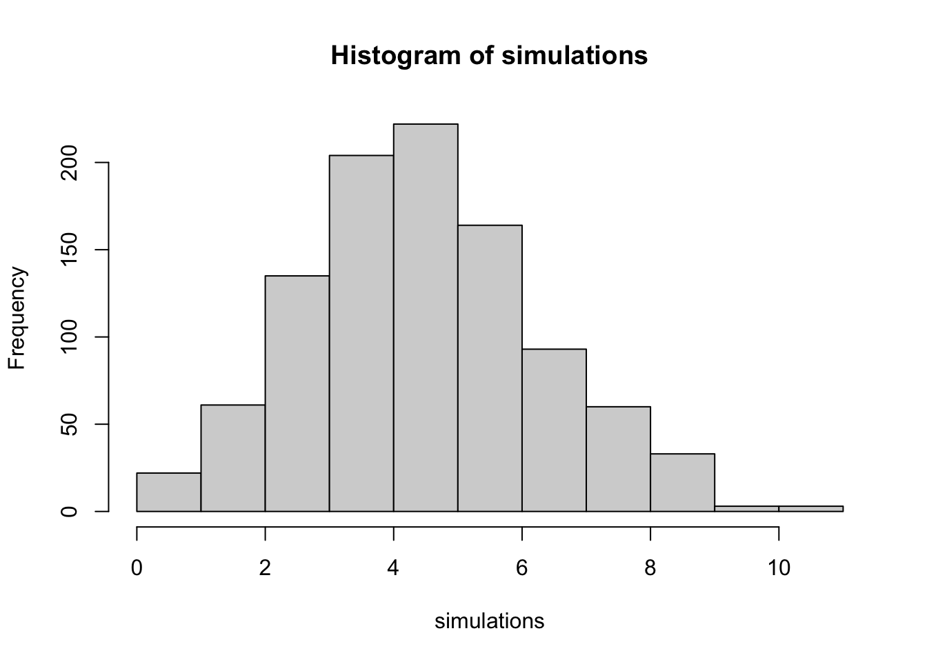

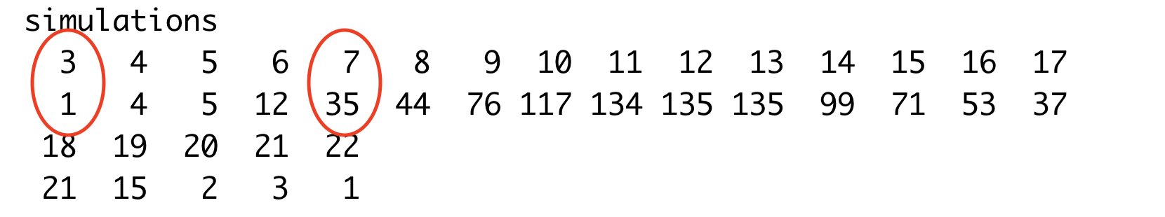
table(simulations)

simulations
  0   1   2   3   4   5   6   7   8   9  10  11 
  5  17  61 135 204 222 164  93  60  33   3   3

Short answer: Pretty weird, but not totally unheard of. If you simulate 15 threes 1000 times, about 17 times it will result in a single made three-pointer. It’s slightly more common that the team would hit 9 threes out of 15. So going that cold is not totally out of the realm of random chance, but it’s pretty rare.

14.2 The hottest of streaks

Last season, Terps baseball player Sam Hojnar hit two home runs in consecutive games. He hit 16 HRs for the season in 233 at-bats, so his home run probability per at-bat was just under seven percent. We’ll use that and the number of games (56) to calculate the odds that he’d hit two home runs in each of two consecutive games.

# Hojnar's statistics
home_runs <- 16
games <- 56
at_bats <- 233

# Calculate probabilities
home_run_prob_per_at_bat <- home_runs / at_bats
avg_at_bats_per_game <- at_bats / games

# Set simulation parameters
num_simulations <- 100000

# Run simulation
set.seed(1234)  # For reproducibility

simulation_results <- tibble(
  sim = 1:num_simulations,
  game1 = rbinom(num_simulations, round(avg_at_bats_per_game), home_run_prob_per_at_bat),
  game2 = rbinom(num_simulations, round(avg_at_bats_per_game), home_run_prob_per_at_bat)
) |>
  mutate(two_hr_each_game = game1 == 2 & game2 == 2)

# Calculate probability
probability <- simulation_results |>
  summarise(prob = mean(two_hr_each_game)) |>
  pull(prob)

# Print results
cat("Estimated probability of hitting exactly two home runs in each of two consecutive games:", format(round(probability, 6), scientific = FALSE))

Estimated probability of hitting exactly two home runs in each of two consecutive games: 0.0007

Let’s parse that code. We set up our simulations as usual, with one change: because this already seems like a pretty rare event, we’re running 100,000 simulations, and we have to calculate the odds for two games, not one. Then we’re looking for results where the number of home runs in both games is two. The simulation_results dataframe shows that 70 times out of 100,000 Hojnar would hit two home runs in consecutive games, based on his own performance. That’s very, very, very unlikely, and quite a hot streak.