library(tidyverse)
library(refinr)
library(janitor)Data Cleaning Part III: Open Refine
Gather ’round kids and let me tell you a tale. Back in the previous century, Los Angeles Times journalists Sara Fritz and Dwight Morris wanted to answer this seemingly simple question: what do political campaigns spend their money on?
While campaigns are required to list a purpose of each expenditure, the problem is that they can choose what words to use. There’s no standard dictionary or drop-down menu to choose from. Want to call that donut purchase “Food”? Sure. What about “Supplies for volunteers”? Works for me. How about “Meals”? Mom might disagree, but the FEC won’t.
In order to answer their initial question, the reporters had to standardize their data. In other words, all food-related purchases had to be labeled “Food”. All travel expenses had to be “Travel”. It took them months - many months - to do this for every federal candidate.
I tell you this because if they had Open Refine, it would have taken them a week or two, not months.
I did data standardization before Open Refine, and every time I think about it, I get mad.
Fortunately (unfortunately?) several columns in the data we’ll work with are flawed in the same way that the LA Times’ data was, so we can do this work in a better, faster way.
We’re going to explore two ways into Open Refine: Through R, and through Open Refine itself.
Refinr, Open Refine in R
What is Open Refine?
Open Refine is a software program that has tools – algorithms – that find small differences in text and helps you fix them quickly. How Open Refine finds those small differences is through something called clustering. The algorithms behind clustering are not exclusive to Open Refine, so they can be used elsewhere.
Enter refinr, a package that contains the same clustering algorithms as Open Refine but all within R. Go ahead and install it if you haven’t already by opening the console and running install.packages("refinr"). Then we can load libraries as we do.
Let’s load that Maryland state government grants and loan data that we’ve been working with, and to make our standardization work easier we’ll change all the grantees to upper-case.
Now let’s try and group and count the number of grants by recipient. To make it a bit more manageable, let’s use another string function from stringr and filter for recipients that start with the uppercase “W” or lowercase “w” using the function str_detect() with a regular expression.
The filter function in the codeblock below says: look in the city column, and pluck out any value that starts with (the “^” symbol means “starts with”) a lowercase “w” OR (the vertical “|”, called a pipe, means OR) an uppercase “W”.
md_grant_loans |>
  group_by(Grantee) |>
  summarise(
    count=n()
  ) |>
  filter(str_detect(Grantee, '^w|^W')) |>
  arrange(Grantee)
# A tibble: 342 × 2
Grantee count
<chr> <int>
1 W. F. DELAUTER & SON, INC. 1
2 W.R. GRACE & CO. 1
3 WABASH MARKETS OF MARYLAND, INC. 1
4 WAGABOUT 1
5 WAH,LLC 1
6 WALBROOK MILL APARTMENTS 1
7 WALDEN SIERRA 1
8 WALDEN SIERRA INC 1
9 WALDEN SIERRA, INC. 31
10 WALDORF ARETE, LLC 1
# ℹ 332 more rowsThere are several problems in this data that will prevent proper grouping and summarizing - you can see multiple versions of “Walden Sierra”, for example. We’ve learned several functions to fix this manually, but that could take awhile.
By using the Open Refine package for R, refinr, our hope is that it can identify and standardize the data with a little more ease.
The first merging technique that’s part of the refinr package we’ll try is the key_collision_merge.
The key collision merge function takes each string and extracts the key parts of it. It then puts every key in a bin based on the keys matching.
One rule you should follow when using this is: do not overwrite your original fields. Always work on a copy. If you overwrite your original field, how will you know if it did the right thing? How can you compare it to your original data? To follow this, I’m going to mutate a new field called clean_city and put the results of key collision merge there.
cleaned_md_grant_loans <- md_grant_loans |>
  mutate(grantee_clean=key_collision_merge(Grantee)) |>
  select(Grantee, grantee_clean, everything())

cleaned_md_grant_loans
# A tibble: 19,482 × 10
Grantee grantee_clean Grantor `Zip Code` `Fiscal Year` Amount Description
<chr> <chr> <chr> <chr> <dbl> <dbl> <chr>
1 PRINCE GEO… PRINCE GEORG… Commer… 20772 2017 1.28e5 Maryland T…
2 ASSOCIATED… ASSOCIATED B… Depart… 21201 2010 9.34e4 Minority O…
3 WESTED/PUB… WESTED/PUBLI… Maryla… 94107-1242 2014 1.61e6 GRANTS FOR…
4 MARYLAND P… MARYLAND PAT… Depart… 21075 2010 2.14e5 Babies Bor…
5 ANACOSTIA … ANACOSTIA WA… Depart… 20710 2017 1.74e5 Payments m…
6 WASHINGTON… WASHINGTON C… Depart… 21740 2009 5.59e4 grant fund…
7 DOMESTIC V… DOMESTIC VIO… Boards… 21045 2014 1.72e5 Domestic V…
8 DACORE INV… DACORE INVES… MD Sma… 20601 2018 1.04e5 Maryland S…
9 MOUNT ST M… MOUNT ST MAR… Maryla… 21727 2015 1.75e6 Sellinger …
10 OLNEY THEA… OLNEY THEATR… Depart… 20830 2010 2.16e5 Grant fund…
# ℹ 19,472 more rows
# ℹ 3 more variables: Category <chr>, `Fiscal Period` <dbl>, Date <chr>To examine changes refinr made, let’s examine the changes it made to cities that start with the letter “W”.
cleaned_md_grant_loans |>
  group_by(Grantee, grantee_clean) |>
  summarise(
    count=n()
  ) |>
  filter(str_detect(Grantee, '^w|^W')) |>
  arrange(Grantee)
`summarise()` has grouped output by 'Grantee'. You can override using the
`.groups` argument.# A tibble: 342 × 3
# Groups: Grantee [342]
Grantee grantee_clean count
<chr> <chr> <int>
1 W. F. DELAUTER & SON, INC. W. F. DELAUTER & SON, INC. 1
2 W.R. GRACE & CO. W.R. GRACE & CO. 1
3 WABASH MARKETS OF MARYLAND, INC. WABASH MARKETS OF MARYLAND, INC. 1
4 WAGABOUT WAGABOUT 1
5 WAH,LLC WAH,LLC 1
6 WALBROOK MILL APARTMENTS WALBROOK MILL APARTMENTS 1
7 WALDEN SIERRA WALDEN SIERRA, INC. 1
8 WALDEN SIERRA INC WALDEN SIERRA, INC. 1
9 WALDEN SIERRA, INC. WALDEN SIERRA, INC. 31
10 WALDORF ARETE, LLC WALDORF ARETE, LLC 1
# ℹ 332 more rowsYou can see several changes on the first page of results, including that refinr consolidated all the Walden Sierra entries into a single one in grantee_clean, which is pretty smart. Other potential changes, grouping together “WALTER’S ART MUSEUM” and “THE WALTERS ART MUSEUM”, didn’t happen. Key collision will do well with different cases, but all of our records are upper case.
There’s another merging algorithim that’s part of refinr that works a bit differently, called n_gram_merge(). Let’s try applying that one.
cleaned_md_grant_loans <- md_grant_loans |>
  mutate(grantee_clean=n_gram_merge(Grantee)) |>
  select(Grantee, grantee_clean, everything())

cleaned_md_grant_loans
# A tibble: 19,482 × 10
Grantee grantee_clean Grantor `Zip Code` `Fiscal Year` Amount Description
<chr> <chr> <chr> <chr> <dbl> <dbl> <chr>
1 PRINCE GEO… PRINCE GEORG… Commer… 20772 2017 1.28e5 Maryland T…
2 ASSOCIATED… ASSOCIATED B… Depart… 21201 2010 9.34e4 Minority O…
3 WESTED/PUB… WESTED/PUBLI… Maryla… 94107-1242 2014 1.61e6 GRANTS FOR…
4 MARYLAND P… MARYLAND PAT… Depart… 21075 2010 2.14e5 Babies Bor…
5 ANACOSTIA … ANACOSTIA WA… Depart… 20710 2017 1.74e5 Payments m…
6 WASHINGTON… WASHINGTON C… Depart… 21740 2009 5.59e4 grant fund…
7 DOMESTIC V… DOMESTIC VIO… Boards… 21045 2014 1.72e5 Domestic V…
8 DACORE INV… DACORE INVES… MD Sma… 20601 2018 1.04e5 Maryland S…
9 MOUNT ST M… MOUNT ST MAR… Maryla… 21727 2015 1.75e6 Sellinger …
10 OLNEY THEA… OLNEY THEATR… Depart… 20830 2010 2.16e5 Grant fund…
# ℹ 19,472 more rows
# ℹ 3 more variables: Category <chr>, `Fiscal Period` <dbl>, Date <chr>To examine changes refinr made with this algorithm, let’s again look at recipients that start with the letter “W”. We see there wasn’t a substantial change from the previous method, and it even missed a few the first method got.
cleaned_md_grant_loans |>
  group_by(Grantee, grantee_clean) |>
  summarise(
    count=n()
  ) |>
  filter(str_detect(Grantee, '^w|^W')) |>
  arrange(Grantee)
`summarise()` has grouped output by 'Grantee'. You can override using the
`.groups` argument.# A tibble: 342 × 3
# Groups: Grantee [342]
Grantee grantee_clean count
<chr> <chr> <int>
1 W. F. DELAUTER & SON, INC. W. F. DELAUTER & SON, INC. 1
2 W.R. GRACE & CO. W.R. GRACE & CO. 1
3 WABASH MARKETS OF MARYLAND, INC. WABASH MARKETS OF MARYLAND, INC. 1
4 WAGABOUT WAGABOUT 1
5 WAH,LLC WAH,LLC 1
6 WALBROOK MILL APARTMENTS WALBROOK MILL APARTMENTS 1
7 WALDEN SIERRA WALDEN SIERRA, INC. 1
8 WALDEN SIERRA INC WALDEN SIERRA, INC. 1
9 WALDEN SIERRA, INC. WALDEN SIERRA, INC. 31
10 WALDORF ARETE, LLC WALDORF ARETE, LLC 1
# ℹ 332 more rowsThis method also made some good changes, but not in every case. No single method will be perfect and often a combination is necessary.
That’s how you use the Open Refine r package, refinr.
Now let’s upload the data to the interactive version of OpenRefine, which really shines at this task.
Manually cleaning data with Open Refine
Open Refine is free software. You should download and install it; the most recent version is 3.6.0. Refinr is great for quick things on smaller datasets that you can check to make sure it’s not up to any mischief.
For bigger datasets, Open Refine is the way to go. And it has a lot more tools than refinr does (by design).
After you install it, run it. (If you are on a Mac it might tell you that it can’t run the program. Go to System Preferences -> Security & Privacy -> General and click “Open Anyway”.) Open Refine works in the browser, and the app spins up a small web server visible only on your computer to interact with it. A browser will pop up automatically.
You first have to import your data into a project. Click the choose files button and upload a csv of the Maryland state grants and loans.

After your data is loaded into the app, you’ll get a screen to look over what the data looks like. On the top right corner, you’ll see a button to create the project. Click that.

Open Refine has many, many tools. We’re going to use one piece of it, as a tool for data cleaning. To learn how to use it, we’re going to clean the “Grantee” field.
First, let’s make a copy of the original Grantee column so that we can preserve the original data while cleaning the new one.
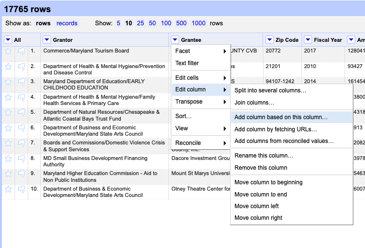
Click the dropdown arrow next to the Grantee column, choose “edit column” > “Add column based on this column”:
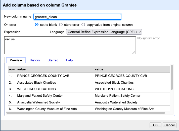
On the window that pops up, type “grantee_clean” in the “new column name” field. Then hit the OK button. We’ll work on that new column.
Now, let’s get to work cleaning the grantee_clean column.
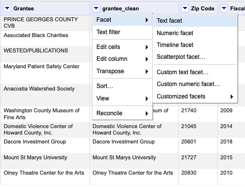
Next to the grantee_clean field name, click the down arrow, then facet, then text facet.
After that, a new box will appear on the left. It tells us how many unique recipient_names there are: 8,956 (you may need to . And, there’s a button on the right of the box that says Cluster.
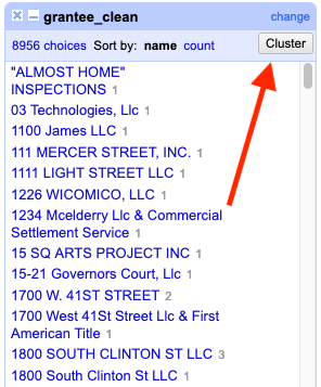
Click the cluster button. A new window will pop up, a tool to help us identify things that need to be cleaned, and quickly clean them.
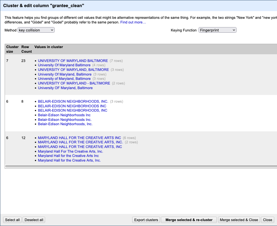
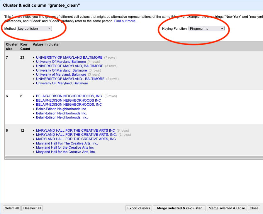
The default “method” used is a clustering algorithim called “key collision”, using the fingerprint function. This is the same method we used with the refinr package above.
At the top, you’ll see which method was used, and how many clusters that algorithm identified. There are several different methods, each of which work slightly differently and produce different results.
Then, below that, you can see what those clusters are. Right away, we can see how useful this program is. It identified 23 rows that have some variation on “University of Maryland - Baltimore” in the grantee_clean field. It proposed changing them all to “UNIVERSITY OF MARYLAND BALTIMORE”.
Using human judgement, you can say if you agree with the cluster. If you do, click the “merge” checkbox. When it merges, the new result will be what it says in New Cell Value. Most often, that’s the row with the most common result. You also can manually edit the “New Cell Value” if you want it to be something else:
Now begins the fun part: You have to look at all the clusters found and decide if they are indeed valid. The key collision method is very good, and very conservative. You’ll find that most of them are usually valid.
Be careful! If you merge two things that aren’t supposed to be together, it will change your data in a way that could lead to inaccurate results.
When you’re done, click Merge Selected and Re-Cluster.
If any new clusters come up, evaluate them. Repeat until either no clusters come up or the clusters that do come up are ones you reject.
Now. Try a new method, maybe the “nearest neighbor levenshtein” method. Notice that it finds even more clusters - using a slightly different approach.
Rinse and repeat.
You’ll keep doing this, and if the dataset is reasonably clean, you’ll find the end.
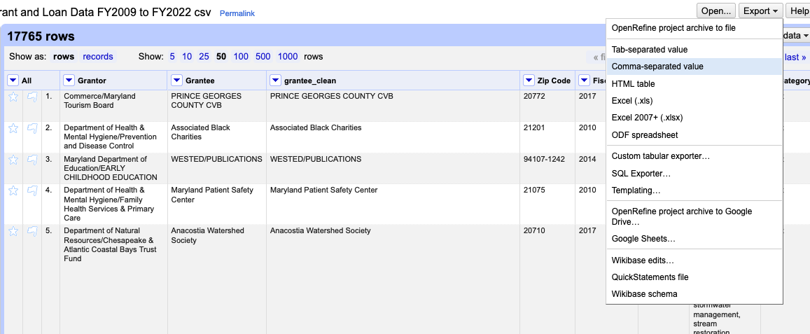
When you’re finished cleaning, click “Merge Selected & Close”.
Then, export the data as a csv so you can load it back into R.
A question for all data analysts – if the dataset is bad enough, can it ever be cleaned?
There’s no good answer. You have to find it yourself.