library(tidyverse)
library(sf)
library(janitor)
library(tigris)
library(tidycensus)
census_api_key("549950d36c22ff16455fe196bbbd01d63cfbe6cf")28 Geographic analysis
In the previous chapter, we looked at election precincts in Prince George’s County to show a bit of a pattern regarding concentration of the precincts with the most and 0 eligible voters. Let’s go little further and look at voters statewide.
First, let’s load the libraries we’ll need, including tigris. We’re also going to load tidycensus and set an API key for tidycensus.
In the previous chapter, we looked at foreclosure notices by zip codes to find patterns in Maryland. Let’s go further and, instead of using raw numbers, use percentages based on the number of owner-occupied housing units in each zip code.
For the rest of this chapter, we’re going to work on building a map that will help us gain insight into geographic patterns in foreclosure notices by county in Maryland. What geographic patterns can we identify?
First, we’ll go out and get the county foreclosure notices and population data for each county using tidycensus. The variable for total population is B01001_001
md_county_notices <- read_csv("data/Maryland_Foreclosure_Data_by_County.csv") |> slice(1) |> pivot_longer(cols=-c('Date', 'Type'), names_to='county', values_to = 'notices')Rows: 63 Columns: 27
── Column specification ────────────────────────────────────────────────────────
Delimiter: ","
chr (2): Date, Type
dbl (25): Allegany County, Anne Arundel County, Baltimore City, Baltimore Co...
ℹ Use `spec()` to retrieve the full column specification for this data.
ℹ Specify the column types or set `show_col_types = FALSE` to quiet this message.md_county_population <- get_acs(geography = "county",
variables = c(population = "B01001_001"),
year = 2021,
state = "MD")Getting data from the 2017-2021 5-year ACSUltimately, we’re going to join this county table with population with foreclosure notices by county, and then calculate a percentage. But remember, we then want to visualize this data by drawing a zip code map that helps us pick out trends. Thinking ahead, we know we’ll need a zip code map shapefile. Fortunately, we can pull this geometry information right from tidycensus at the same time that we pull in the population data by adding “geometry = TRUE” to our get_acs function.
md_county_population <- get_acs(geography = "county",
              variables = c(population = "B01001_001"),
              year = 2021,
              state = "MD",
              geometry = TRUE)
Getting data from the 2017-2021 5-year ACSDownloading feature geometry from the Census website. To cache shapefiles for use in future sessions, set `options(tigris_use_cache = TRUE)`.
|
| | 0%
|
| | 1%
|
|= | 1%
|
|= | 2%
|
|== | 2%
|
|== | 3%
|
|=== | 4%
|
|=== | 5%
|
|==== | 5%
|
|==== | 6%
|
|===== | 6%
|
|===== | 7%
|
|===== | 8%
|
|====== | 8%
|
|====== | 9%
|
|======= | 9%
|
|======= | 10%
|
|======= | 11%
|
|======== | 11%
|
|======== | 12%
|
|========= | 12%
|
|========= | 13%
|
|========= | 14%
|
|========== | 14%
|
|========== | 15%
|
|=========== | 15%
|
|=========== | 16%
|
|============ | 17%
|
|============ | 18%
|
|============= | 18%
|
|============= | 19%
|
|============== | 19%
|
|============== | 20%
|
|============== | 21%
|
|=============== | 21%
|
|=============== | 22%
|
|================ | 22%
|
|================ | 23%
|
|================= | 24%
|
|================= | 25%
|
|================== | 25%
|
|================== | 26%
|
|=================== | 27%
|
|=================== | 28%
|
|==================== | 28%
|
|==================== | 29%
|
|===================== | 29%
|
|===================== | 30%
|
|===================== | 31%
|
|====================== | 31%
|
|====================== | 32%
|
|======================= | 32%
|
|======================= | 33%
|
|======================= | 34%
|
|======================== | 34%
|
|======================== | 35%
|
|========================= | 35%
|
|========================= | 36%
|
|========================== | 36%
|
|========================== | 37%
|
|========================== | 38%
|
|=========================== | 38%
|
|=========================== | 39%
|
|============================ | 39%
|
|============================ | 40%
|
|============================ | 41%
|
|============================= | 41%
|
|============================= | 42%
|
|============================== | 42%
|
|============================== | 43%
|
|=============================== | 44%
|
|=============================== | 45%
|
|================================ | 45%
|
|================================ | 46%
|
|================================= | 47%
|
|================================= | 48%
|
|================================== | 48%
|
|================================== | 49%
|
|=================================== | 49%
|
|=================================== | 50%
|
|=================================== | 51%
|
|==================================== | 51%
|
|==================================== | 52%
|
|===================================== | 52%
|
|===================================== | 53%
|
|===================================== | 54%
|
|====================================== | 54%
|
|====================================== | 55%
|
|======================================= | 55%
|
|======================================= | 56%
|
|======================================== | 56%
|
|======================================== | 57%
|
|======================================== | 58%
|
|========================================= | 58%
|
|========================================= | 59%
|
|========================================== | 59%
|
|========================================== | 60%
|
|========================================== | 61%
|
|=========================================== | 61%
|
|=========================================== | 62%
|
|============================================ | 62%
|
|============================================ | 63%
|
|============================================ | 64%
|
|============================================= | 64%
|
|============================================= | 65%
|
|============================================== | 65%
|
|============================================== | 66%
|
|=============================================== | 67%
|
|=============================================== | 68%
|
|================================================ | 68%
|
|================================================ | 69%
|
|================================================= | 69%
|
|================================================= | 70%
|
|================================================= | 71%
|
|================================================== | 71%
|
|================================================== | 72%
|
|=================================================== | 72%
|
|=================================================== | 73%
|
|==================================================== | 74%
|
|==================================================== | 75%
|
|===================================================== | 75%
|
|===================================================== | 76%
|
|====================================================== | 76%
|
|====================================================== | 77%
|
|====================================================== | 78%
|
|======================================================= | 78%
|
|======================================================= | 79%
|
|======================================================== | 79%
|
|======================================================== | 80%
|
|======================================================== | 81%
|
|========================================================= | 81%
|
|========================================================= | 82%
|
|========================================================== | 82%
|
|========================================================== | 83%
|
|========================================================== | 84%
|
|=========================================================== | 84%
|
|=========================================================== | 85%
|
|============================================================ | 85%
|
|============================================================ | 86%
|
|============================================================= | 87%
|
|============================================================= | 88%
|
|============================================================== | 88%
|
|============================================================== | 89%
|
|=============================================================== | 89%
|
|=============================================================== | 90%
|
|=============================================================== | 91%
|
|================================================================ | 91%
|
|================================================================ | 92%
|
|================================================================= | 92%
|
|================================================================= | 93%
|
|================================================================== | 94%
|
|================================================================== | 95%
|
|=================================================================== | 95%
|
|=================================================================== | 96%
|
|==================================================================== | 97%
|
|==================================================================== | 98%
|
|===================================================================== | 98%
|
|===================================================================== | 99%
|
|======================================================================| 99%
|
|======================================================================| 100%md_county_populationSimple feature collection with 24 features and 5 fields
Geometry type: MULTIPOLYGON
Dimension: XY
Bounding box: xmin: -79.48765 ymin: 37.91172 xmax: -75.04894 ymax: 39.72304
Geodetic CRS: NAD83
First 10 features:
GEOID NAME variable estimate moe
1 24047 Worcester County, Maryland population 52322 NA
2 24003 Anne Arundel County, Maryland population 584064 NA
3 24033 Prince George's County, Maryland population 957767 NA
4 24025 Harford County, Maryland population 259162 NA
5 24015 Cecil County, Maryland population 103370 NA
6 24011 Caroline County, Maryland population 33234 NA
7 24023 Garrett County, Maryland population 28955 NA
8 24029 Kent County, Maryland population 19335 NA
9 24041 Talbot County, Maryland population 37510 NA
10 24045 Wicomico County, Maryland population 103223 NA
geometry
1 MULTIPOLYGON (((-75.66061 3...
2 MULTIPOLYGON (((-76.83849 3...
3 MULTIPOLYGON (((-77.07995 3...
4 MULTIPOLYGON (((-76.0921 39...
5 MULTIPOLYGON (((-76.23326 3...
6 MULTIPOLYGON (((-76.01505 3...
7 MULTIPOLYGON (((-79.48765 3...
8 MULTIPOLYGON (((-76.27737 3...
9 MULTIPOLYGON (((-76.34647 3...
10 MULTIPOLYGON (((-75.92033 3...We now have a new column, geometry, that contains the “MULTIPOLYGON” data that will draw an outline of each county when we go to draw a map.
The next step will be to join our population data to our foreclosure data on the county column.
But there’s a problem. The column in our population data that has county names is called “NAME”, and it has the full name of the county spelled out in title case – first word capitalized and has “County” and “Maryland” in it. The foreclosure data just has the name of the county. For example, the population data has “Anne Arundel County, Maryland” and the foreclosure data has “Anne Arundel County”.
md_county_populationSimple feature collection with 24 features and 5 fields
Geometry type: MULTIPOLYGON
Dimension: XY
Bounding box: xmin: -79.48765 ymin: 37.91172 xmax: -75.04894 ymax: 39.72304
Geodetic CRS: NAD83
First 10 features:
GEOID NAME variable estimate moe
1 24047 Worcester County, Maryland population 52322 NA
2 24003 Anne Arundel County, Maryland population 584064 NA
3 24033 Prince George's County, Maryland population 957767 NA
4 24025 Harford County, Maryland population 259162 NA
5 24015 Cecil County, Maryland population 103370 NA
6 24011 Caroline County, Maryland population 33234 NA
7 24023 Garrett County, Maryland population 28955 NA
8 24029 Kent County, Maryland population 19335 NA
9 24041 Talbot County, Maryland population 37510 NA
10 24045 Wicomico County, Maryland population 103223 NA
geometry
1 MULTIPOLYGON (((-75.66061 3...
2 MULTIPOLYGON (((-76.83849 3...
3 MULTIPOLYGON (((-77.07995 3...
4 MULTIPOLYGON (((-76.0921 39...
5 MULTIPOLYGON (((-76.23326 3...
6 MULTIPOLYGON (((-76.01505 3...
7 MULTIPOLYGON (((-79.48765 3...
8 MULTIPOLYGON (((-76.27737 3...
9 MULTIPOLYGON (((-76.34647 3...
10 MULTIPOLYGON (((-75.92033 3...md_county_notices# A tibble: 25 × 4
Date Type county notices
<chr> <chr> <chr> <dbl>
1 03/01/2023 12:00:00 AM Notice of Intent to Foreclose Allegany County 79
2 03/01/2023 12:00:00 AM Notice of Intent to Foreclose Anne Arundel Co… 475
3 03/01/2023 12:00:00 AM Notice of Intent to Foreclose Baltimore City 754
4 03/01/2023 12:00:00 AM Notice of Intent to Foreclose Baltimore County 847
5 03/01/2023 12:00:00 AM Notice of Intent to Foreclose Calvert County 116
6 03/01/2023 12:00:00 AM Notice of Intent to Foreclose Caroline County 40
7 03/01/2023 12:00:00 AM Notice of Intent to Foreclose Carroll County 133
8 03/01/2023 12:00:00 AM Notice of Intent to Foreclose Cecil County 109
9 03/01/2023 12:00:00 AM Notice of Intent to Foreclose Charles County 336
10 03/01/2023 12:00:00 AM Notice of Intent to Foreclose Dorchester Coun… 41
# ℹ 15 more rowsIf they’re going to join properly, we need to clean one of them up to make it match the other.
Let’s clean the population table. We’re going to rename the “NAME” column to “County”, then remove “, Maryland” and “County” and make the county titlecase. Next we’ll remove any white spaces after that first cleaning step that, if left in, would prevent a proper join. We’re also going to rename the column that contains the population information from “estimate” to “population” and select only the county name and the population columns, along with the geometry. That leaves us with this tidy table.
md_county_population <- md_county_population |>
  rename(county = NAME) |>
  mutate(county = str_to_title(str_remove_all(county,", Maryland"))) |>
  mutate(county = str_trim(county,side="both")) |>
  rename(population = estimate) |>
  select(county, population, geometry)

md_county_population
Simple feature collection with 24 features and 2 fields
Geometry type: MULTIPOLYGON
Dimension: XY
Bounding box: xmin: -79.48765 ymin: 37.91172 xmax: -75.04894 ymax: 39.72304
Geodetic CRS: NAD83
First 10 features:
county population geometry
1 Worcester County 52322 MULTIPOLYGON (((-75.66061 3...
2 Anne Arundel County 584064 MULTIPOLYGON (((-76.83849 3...
3 Prince George's County 957767 MULTIPOLYGON (((-77.07995 3...
4 Harford County 259162 MULTIPOLYGON (((-76.0921 39...
5 Cecil County 103370 MULTIPOLYGON (((-76.23326 3...
6 Caroline County 33234 MULTIPOLYGON (((-76.01505 3...
7 Garrett County 28955 MULTIPOLYGON (((-79.48765 3...
8 Kent County 19335 MULTIPOLYGON (((-76.27737 3...
9 Talbot County 37510 MULTIPOLYGON (((-76.34647 3...
10 Wicomico County 103223 MULTIPOLYGON (((-75.92033 3...Now we can join them.
md_pop_with_foreclosures <- md_county_population |>
  left_join(md_county_notices, join_by(county))

md_pop_with_foreclosures
Simple feature collection with 24 features and 5 fields
Geometry type: MULTIPOLYGON
Dimension: XY
Bounding box: xmin: -79.48765 ymin: 37.91172 xmax: -75.04894 ymax: 39.72304
Geodetic CRS: NAD83
First 10 features:
county population Date
1 Worcester County 52322 03/01/2023 12:00:00 AM
2 Anne Arundel County 584064 03/01/2023 12:00:00 AM
3 Prince George's County 957767 03/01/2023 12:00:00 AM
4 Harford County 259162 03/01/2023 12:00:00 AM
5 Cecil County 103370 03/01/2023 12:00:00 AM
6 Caroline County 33234 03/01/2023 12:00:00 AM
7 Garrett County 28955 03/01/2023 12:00:00 AM
8 Kent County 19335 03/01/2023 12:00:00 AM
9 Talbot County 37510 03/01/2023 12:00:00 AM
10 Wicomico County 103223 03/01/2023 12:00:00 AM
Type notices geometry
1 Notice of Intent to Foreclose 47 MULTIPOLYGON (((-75.66061 3...
2 Notice of Intent to Foreclose 475 MULTIPOLYGON (((-76.83849 3...
3 Notice of Intent to Foreclose 1389 MULTIPOLYGON (((-77.07995 3...
4 Notice of Intent to Foreclose 250 MULTIPOLYGON (((-76.0921 39...
5 Notice of Intent to Foreclose 109 MULTIPOLYGON (((-76.23326 3...
6 Notice of Intent to Foreclose 40 MULTIPOLYGON (((-76.01505 3...
7 Notice of Intent to Foreclose 13 MULTIPOLYGON (((-79.48765 3...
8 Notice of Intent to Foreclose 19 MULTIPOLYGON (((-76.27737 3...
9 Notice of Intent to Foreclose 22 MULTIPOLYGON (((-76.34647 3...
10 Notice of Intent to Foreclose 68 MULTIPOLYGON (((-75.92033 3...Our final step before visualization, let’s calculate the number of foreclosure notices per 1000 population and sort from highest to lowest to see what trends we can identify just from the table.
md_pop_with_foreclosures <- md_county_population |>
  left_join(md_county_notices, join_by(county)) |>
  mutate(rate = notices/population*1000) |>
  arrange(desc(rate))

md_pop_with_foreclosures
Simple feature collection with 24 features and 6 fields
Geometry type: MULTIPOLYGON
Dimension: XY
Bounding box: xmin: -79.48765 ymin: 37.91172 xmax: -75.04894 ymax: 39.72304
Geodetic CRS: NAD83
First 10 features:
county population Date
1 Charles County 165209 03/01/2023 12:00:00 AM
2 Prince George's County 957767 03/01/2023 12:00:00 AM
3 Baltimore City 592211 03/01/2023 12:00:00 AM
4 Dorchester County 32486 03/01/2023 12:00:00 AM
5 Calvert County 92515 03/01/2023 12:00:00 AM
6 Caroline County 33234 03/01/2023 12:00:00 AM
7 Allegany County 68684 03/01/2023 12:00:00 AM
8 Cecil County 103370 03/01/2023 12:00:00 AM
9 St. Mary's County 113209 03/01/2023 12:00:00 AM
10 Baltimore County 850702 03/01/2023 12:00:00 AM
Type notices rate
1 Notice of Intent to Foreclose 336 2.0337875
2 Notice of Intent to Foreclose 1389 1.4502483
3 Notice of Intent to Foreclose 754 1.2731949
4 Notice of Intent to Foreclose 41 1.2620821
5 Notice of Intent to Foreclose 116 1.2538507
6 Notice of Intent to Foreclose 40 1.2035867
7 Notice of Intent to Foreclose 79 1.1501951
8 Notice of Intent to Foreclose 109 1.0544645
9 Notice of Intent to Foreclose 113 0.9981539
10 Notice of Intent to Foreclose 847 0.9956483
geometry
1 MULTIPOLYGON (((-77.27382 3...
2 MULTIPOLYGON (((-77.07995 3...
3 MULTIPOLYGON (((-76.71152 3...
4 MULTIPOLYGON (((-76.06544 3...
5 MULTIPOLYGON (((-76.70121 3...
6 MULTIPOLYGON (((-76.01505 3...
7 MULTIPOLYGON (((-79.06756 3...
8 MULTIPOLYGON (((-76.23326 3...
9 MULTIPOLYGON (((-76.74729 3...
10 MULTIPOLYGON (((-76.3257 39...Let’s take a look at the result of this table. The variances in the rates aren’t huge, but there are some clear differences: Charles County and Prince George’s County have higher rates, followed by Baltimore City and some more rural counties.
First, let’s use the counties() function from tigris to pull down a shapefile of all U.S. counties and grab the ones for Maryland.
md_counties <- counties() |>
  filter(STATEFP == "24")
Retrieving data for the year 2022
|
| | 0%
|
| | 1%
|
|= | 1%
|
|= | 2%
|
|== | 2%
|
|== | 3%
|
|== | 4%
|
|=== | 4%
|
|=== | 5%
|
|==== | 5%
|
|==== | 6%
|
|===== | 6%
|
|===== | 7%
|
|===== | 8%
|
|====== | 8%
|
|====== | 9%
|
|======= | 9%
|
|======= | 10%
|
|======= | 11%
|
|======== | 11%
|
|======== | 12%
|
|========= | 12%
|
|========= | 13%
|
|========= | 14%
|
|========== | 14%
|
|========== | 15%
|
|=========== | 15%
|
|=========== | 16%
|
|============ | 16%
|
|============ | 17%
|
|============ | 18%
|
|============= | 18%
|
|============= | 19%
|
|============== | 19%
|
|============== | 20%
|
|============== | 21%
|
|=============== | 21%
|
|=============== | 22%
|
|================ | 22%
|
|================ | 23%
|
|================ | 24%
|
|================= | 24%
|
|================= | 25%
|
|================== | 25%
|
|================== | 26%
|
|=================== | 26%
|
|=================== | 27%
|
|=================== | 28%
|
|==================== | 28%
|
|==================== | 29%
|
|===================== | 29%
|
|===================== | 30%
|
|===================== | 31%
|
|====================== | 31%
|
|====================== | 32%
|
|======================= | 32%
|
|======================= | 33%
|
|======================= | 34%
|
|======================== | 34%
|
|======================== | 35%
|
|========================= | 35%
|
|========================= | 36%
|
|========================== | 36%
|
|========================== | 37%
|
|========================== | 38%
|
|=========================== | 38%
|
|=========================== | 39%
|
|============================ | 39%
|
|============================ | 40%
|
|============================ | 41%
|
|============================= | 41%
|
|============================= | 42%
|
|============================== | 42%
|
|============================== | 43%
|
|============================== | 44%
|
|=============================== | 44%
|
|=============================== | 45%
|
|================================ | 45%
|
|================================ | 46%
|
|================================= | 46%
|
|================================= | 47%
|
|================================= | 48%
|
|================================== | 48%
|
|================================== | 49%
|
|=================================== | 49%
|
|=================================== | 50%
|
|=================================== | 51%
|
|==================================== | 51%
|
|==================================== | 52%
|
|===================================== | 52%
|
|===================================== | 53%
|
|===================================== | 54%
|
|====================================== | 54%
|
|====================================== | 55%
|
|======================================= | 55%
|
|======================================= | 56%
|
|======================================== | 56%
|
|======================================== | 57%
|
|======================================== | 58%
|
|========================================= | 58%
|
|========================================= | 59%
|
|========================================== | 59%
|
|========================================== | 60%
|
|========================================== | 61%
|
|=========================================== | 61%
|
|=========================================== | 62%
|
|============================================ | 62%
|
|============================================ | 63%
|
|============================================ | 64%
|
|============================================= | 64%
|
|============================================= | 65%
|
|============================================== | 65%
|
|============================================== | 66%
|
|=============================================== | 66%
|
|=============================================== | 67%
|
|=============================================== | 68%
|
|================================================ | 68%
|
|================================================ | 69%
|
|================================================= | 69%
|
|================================================= | 70%
|
|================================================= | 71%
|
|================================================== | 71%
|
|================================================== | 72%
|
|=================================================== | 72%
|
|=================================================== | 73%
|
|=================================================== | 74%
|
|==================================================== | 74%
|
|==================================================== | 75%
|
|===================================================== | 75%
|
|===================================================== | 76%
|
|====================================================== | 76%
|
|====================================================== | 77%
|
|====================================================== | 78%
|
|======================================================= | 78%
|
|======================================================= | 79%
|
|======================================================== | 79%
|
|======================================================== | 80%
|
|======================================================== | 81%
|
|========================================================= | 81%
|
|========================================================= | 82%
|
|========================================================== | 82%
|
|========================================================== | 83%
|
|========================================================== | 84%
|
|=========================================================== | 84%
|
|=========================================================== | 85%
|
|============================================================ | 85%
|
|============================================================ | 86%
|
|============================================================= | 86%
|
|============================================================= | 87%
|
|============================================================= | 88%
|
|============================================================== | 88%
|
|============================================================== | 89%
|
|=============================================================== | 89%
|
|=============================================================== | 90%
|
|=============================================================== | 91%
|
|================================================================ | 91%
|
|================================================================ | 92%
|
|================================================================= | 92%
|
|================================================================= | 93%
|
|================================================================= | 94%
|
|================================================================== | 94%
|
|================================================================== | 95%
|
|=================================================================== | 95%
|
|=================================================================== | 96%
|
|==================================================================== | 96%
|
|==================================================================== | 97%
|
|==================================================================== | 98%
|
|===================================================================== | 98%
|
|===================================================================== | 99%
|
|======================================================================| 99%
|
|======================================================================| 100%Okay, now let’s visualize. We’re going to build a choropleth map, with the color of each county – the fill – set according to the number of notices per 1K population on a color gradient.
county_centroids <- st_centroid(md_counties)Warning: st_centroid assumes attributes are constant over geometriescounty_centroids_df <- as.data.frame(st_coordinates(county_centroids))
county_centroids_df$NAME <- county_centroids$NAME
ggplot() +
geom_sf(data=md_pop_with_foreclosures, aes(fill=rate)) +
geom_text(aes(x = X, y = Y, label = NAME), data = county_centroids_df, size = 3, check_overlap = TRUE) +
theme_minimal()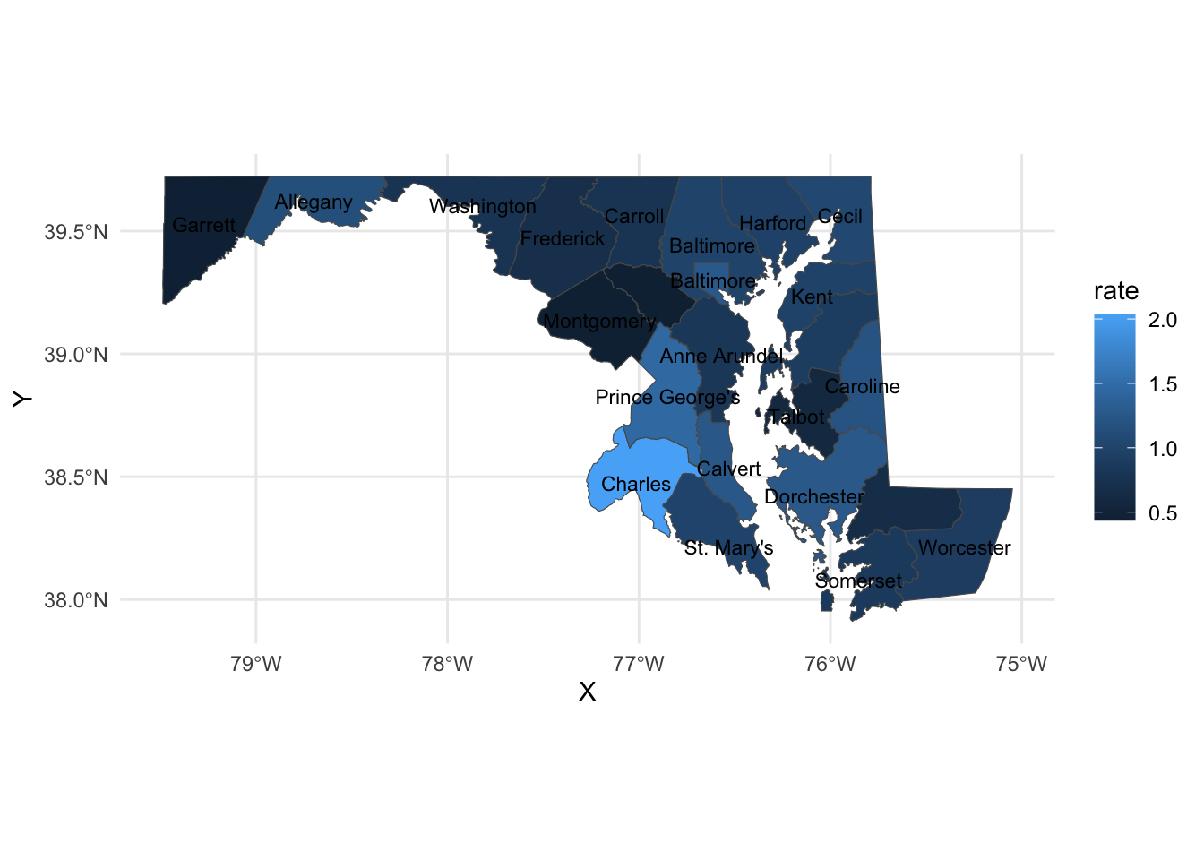
This map is okay, but the color scale makes it hard to draw fine-grained differences. Let’s try applying the magma color scale we learned in the last chapter.
ggplot() +
  geom_sf(data=md_pop_with_foreclosures, aes(fill=rate)) +
  theme_minimal() +
  scale_fill_viridis_b(option="magma")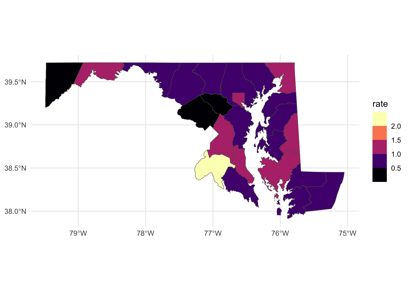
The highest ranking counties stand out nicely in this version, but it’s still hard to make out fine-grained differences between other counties.
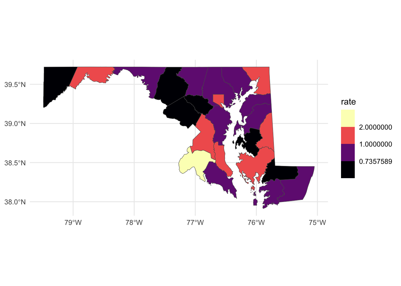
So let’s change the color scale to a “log” scale, which will help us see those differences a bit more clearly.
ggplot() +
  geom_sf(data=md_pop_with_foreclosures, aes(fill=rate)) +
  theme_minimal() +
  scale_fill_viridis_b(option="magma",trans = "log")